Algorithm

Consider the linear regression with samples (y_1,x_1), (y_2,x_2), cdots, (y_n,x_n) satisfying:

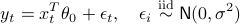
$y_t = x_t^T theta_0+ epsilon_t, quad epsilon_i stackrel{rm{iid}}{sim}{sf N}(0,sigma^2)$

Here $theta_0in mathbb{R}^p$ is an unknown parameter vector relating the covariates x_t to the response y_t , and epsilon_t are noise terms. ‘‘The covariates are potentially collected adaptively, and so can be correlated to prior covariates $x_1, x_2, dotsc, x_{t-1}$ .’’

Goal: We aim at ex post statistical inference on individual model parameters $theta_{0,t}$ , in terms of frequentist p-value and confidence interval.

Method

Below we provide a brief explanation of the online debiasing method. For more details and scissions, we refer to our paper.

Denote by 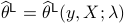$widehat{theta}^{sf L} = widehat{theta}^{sf L}(y,X;lambda)$ the Lasso estimator

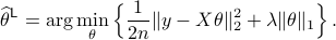
$widehat{theta}^{sf L} = argmin_{theta} Big{frac{1}{2n} |y-Xtheta|_2^2 + lambda |theta|_1 Big},.$

The online debased estimator $widehat{theta}^{sf on} = widehat{theta}^{sf on}(y,X;(M_t)_{tle n}, lambda)$ takes the form

$widehat{theta}^{sf on} := widehat{theta}^{sf L} + frac{1}{n}sum_{t=1}^n M_t x_t (y_t -x_t^Twidehat{theta}^{sf L})$

The term ‘online’ comes from the crucial constraint of predictability imposed on the sequence: there exists a filtration $({frak{F}}_t)_{tge 0}$ so that, (1) epsilon_t are adapted to $({frak{F}})_t$ and is independent of ${frak{F}}_s$ for s< t . We assume that the sequences $(x_t)_{tge 1}$ and $(M_t)_{tge 1}$ are predictable with respect to ${frak{F}}_t$ .

How to choose decorrelating matrices?

We focus on times series as an important application of adaptively collected data and consider a vector autoregression (VAR) model for time series. By a proper change of variables, a Var(d) model can be represented as the linear regression with dp^2 parameters and n = T-d sample size where is the time horizon where we observe the times series, and is the lag. Our primary interest is in high-dimensional Var(d) model, where the number of model parameters dp^2 exceeds the sample size n = T-d .

The proposed online debiasing provides valid statistical significance measures for the model parameters (the time invariant matrices in the Var(d) model).

To construct decorrelating matrices M_i that satisfy the predictability condition, we proceed as follows:

For given positive integer numbers $r_0, r_1, dotsc, r_{K-1}$ that add up to , we partition the time horizon into episodes $E_0, E_1, dotsc, E_{K-1}$ , with of length and let $widehat{Sigma}^{(ell)}$ be the sample covariance of features in the first episodes.

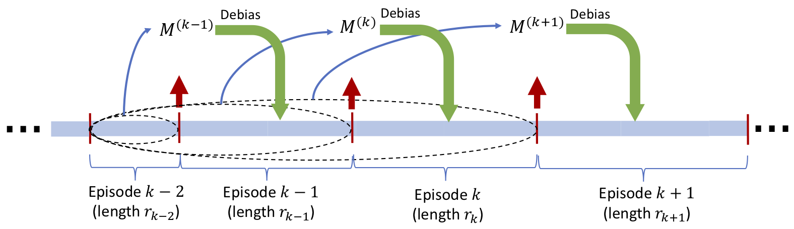At the beginning of each episode , we calculate a decorrelating matrix $M^{(ell)}$ using the previous data points and use that matrix to debias the sample coming in the current episode, that is to say $M_t = M^{(ell)}$ for $tin E_{ell}$ . The details of this step are summarized in the box below.

1. For a = 1,2,dotsc, dp do Construct $m^ell_ain mathbb{R}^{dp}$ by solving the following optimization:

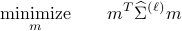
$underset{m}{text{minimize}} quadquad m^T widehat{Sigma}^{(ell)} m$

$text{subject to}quad, |widehat{Sigma}^{ell} m - e_a|_infty le mu, quad |m|_1le L,,$

With e_a the standard basis element with one at the -th position and zero everywhere else.

2. Set $M^{(ell)} = (m^ell_1, m^ell_2, dotsc, m^ell_{dp})^T$ . In words, stack the constructed vectors m^ell_a as rows of $M^{(ell)}$ .

Our analysis in the paper suggests the choice of episode lengths r_ellsim alpha^ell . The code can take the parameter alpha as an input.